

Introduction
Today, as artificial intelligence continues to advance at an unprecedented pace, we stand on the brink of a technological revolution - one driven by machine learning, predictive algorithms and massive data ecosystems that are reshaping our world in ways once confined to science fiction.
Yet, AI is only as powerful as the data that fuels it. When that data is incomplete, historically biased, or lacks diversity, the outcomes can be deeply flawed, even harmful. In many cases, this means amplifying the very discrimination AI was meant to eliminate.
A striking example lies in the hiring space: Following the release of the first diversity reports in 2014, which exposed the underrepresentation of women in tech, many organizations turned to AI-driven hiring tools to reduce "human bias". Yet, without proper checks, these systems ended up mirroring the same prejudices embedded in past hiring data - a classic case of "garbage in, garbage out." In essence, algorithms trained on biased data learned to replicate historical discrimination rather than correct it.
In this blog, we'll uncover how bias seeps into AI systems, why it's so challenging to detect and the tangible impact it has on real lives. More importantly, we'll explore practical ways to design AI that is fair, transparent and truly inclusive.
AI's Double-Edged Nature
AI is now embedded in critical decision-making pipelines across industries like healthcare, hiring, finance, law enforcement and beyond. It is in systems that decide who gets a loan, who gets hired, what medical treatment is recommended and even who gets flagged for police attention. AI brings speed, efficiency and predictive power to processes once limited by human capacity. However as the saying goes "With great power comes great responsibility".
Here's the contradiction:
- AI doesn't have intent, but it does have impact.
- AI doesn't hate or discriminate, but it can learn patterns from data that reflect our society's inequalities and amplify them.
A simple rule captures the complicacy in a nut shell: A biased dataset → a biased model → biased outcomes.
It's the digital version of the old saying: "You are what you eat". For AI, the "diet" is data and when that diet is unbalanced, the system's decisions can turn toxic.
How Data Bias Happens
Bias isn't always malicious — it's often invisible, buried deep in the data collection and preparation process. Let's break down the most common sources:
Incomplete Data or Sampling Bias
Incomplete data means entire populations are underrepresented. This can lead to systematic misclassification or neglect of certain groups.
For example: In Google Photos Mislabeling Incident (2015), Google's image recognition system famously misclassified photos of Black people as gorillas. This happened because the facial recognition model had been trained primarily on lighter-skinned faces, with very few images of darker skin tones in its dataset. Because the AI had limited examples of Black faces, it could not accurately distinguish features leading to a deeply offensive and harmful error.
Historical Bias
Data often reflects history, not fairness. Even without overt prejudice, past discrimination becomes encoded in future predictions.
For example: Banks historically offered fewer loans in minority or low-income areas, leading to sparse credit history for residents. AI models trained on this data may unfairly assign lower credit scores to these individuals, even if their current financial behavior is strong. This replicates historical inequities without any explicit discrimination in the algorithm itself.
Improper Data Partitioning
Even the way we split data can introduce bias. If the train-test split isn't stratified meaning not all demographic groups are fairly represented in both, the model might never see certain categories during training. It will then face "unknown" data during deployment and perform poorly for those groups.
Synthetic Data Pitfalls
Synthetic data are artificially generated samples meant to expand datasets, they are a promising solution for privacy and diversity issues. But when poorly generated, it can distort reality.
For instance, a model trained on synthetic medical images might not capture the nuanced variations of real patients. When deployed in hospitals, it can make dangerous misclassifications.
Bias doesn't need to be deliberate; sometimes, it's as simple as who had access to the data and who didn't.
Real-World Impact: When Biased AI Hurts People
The abstract concept of "data bias" becomes frighteningly real when lives, careers, or rights are at stake. Let's look at some landmark cases.
1. Healthcare: When Cost Became the Proxy for Care
In 2019, a study revealed racial bias in a healthcare algorithm designed to identify patients who needed extra medical attention. Led by Ziad Obermeyer at UC Berkeley, the study found that Black patients, despite being equally or more ill, were often excluded from high-risk care. It used historical healthcare spending as an indicator of illness severity. But because Black patients historically spend less on healthcare (due to systemic inequities, not better health), the algorithm concluded they were healthier than they actually were. Only 17.7% of Black patients were selected for support, a number that could have risen to 46.5% with a fairer algorithm.
2. Recruitment: Amazon's Gender Bias Model
Amazon once built an internal AI tool to automate resume screening. It was trained on a decade's worth of applications but from a predominantly male tech workforce. Unsurprisingly, the system began downgrading applications containing the word "women's" (as in "women's chess club captain") and preferred resumes with more masculine-coded language. Amazon eventually scrapped the project, acknowledging that the algorithm had learned gender bias directly from historical data.
3. Synthetic Data Failure: IBM Watson for Oncology
IBM Watson was once hailed as the future of AI in medicine. However, its oncology recommendation system faced criticism after reports surfaced that it provided incorrect and unsafe treatment recommendations. This shortcoming was due, in part, to Watson's reliance on "synthetic" data and hypothetical cases rather than real-world patient data. By training on artificial cases the system's recommendations risked misaligning with real-world medical needs, endangering patient health. Dr. Jonathan Chen, an assistant professor at Stanford's Center for Biomedical Informatic Research said "I would certainly want to see some validation to whether the synthetic data is representative of anything that would make sense".
These examples illustrate the "garbage in, garbage out" principle. When the input data is biased or incomplete, no amount of sophisticated modeling can save the output from being wrong or worse, harmful
Building Better AI: A Practical Toolkit
1. Data Strategies
-
Keep a Domain Expert on the Team: Ensure at least one domain expert is involved throughout the data lifecycle, from collection to model validation. Their contextual knowledge helps identify hidden biases, validate assumptions and interpret results accurately.
-
Collect Diverse and Representative Datasets: Proactively gather data from multiple demographics, geographies and socioeconomic backgrounds. In healthcare, that means including patients of different ages, ethnicities and income levels. In finance, it means reflecting customers from varied income brackets, not just those with stable credit histories.
-
Validate Synthetic Data Distributions: Synthetic data can enhance privacy and fill data gaps, but only when properly validated. Before deployment, confirm that its statistical patterns align with real-world distributions to maintain fairness and reliability.
2. Data Validation & Integrity
Before even checking for fairness, we need to ensure that our training and testing data represent the same population. A biased split can silently skew model performance long before deployment. Here's a quick cheat sheet for validating data splits:
| Metric / Test | Feature Type | What It Checks | Interpretation / Threshold | When to Use |
|---|---|---|---|---|
| Mean and Std Comparison | Numerical | Central tendency and spread | Mean or std diff greater than 10% indicates splits may not represent the same population | Baseline numerical check |
| Category Proportion Difference | Categorical | Category frequencies | Category share diff greater than 10% suggests imbalance | Simple frequency check |
| Kolmogorov-Smirnov Test | Numerical | Distribution similarity | p > 0.05 = similar, p < 0.05 = potential drift | Continuous features |
| Population Stability Index | Numerical / Categorical | Feature drift magnitude | < 0.1 = stable; 0.1–0.25 = moderate drift; > 0.25 = concerning | Continuous or categorical drift monitoring |
| Cramer's V | Categorical | Association with dataset split | Low values = independence (good); high values = split bias | Detects categorical distribution bias |
| Chi-Square Test | Categorical | Category proportion similarity | p > 0.05 = frequencies similar | Nominal categorical features |
| Correlation Matrix Comparison | Mixed | Relationship consistency | Correlation difference < 0.1 recommended | Ensures relationships remain consistent |
3. Model Fairness Auditing
Even with clean, balanced data, bias can creep back in during model training and evaluation. Algorithms learn patterns and if those patterns encode historical prejudice or sampling imbalance, the model may make systematically unfair predictions. That's why fairness auditing is critical after the model is built, not just before. Here's how to do it effectively:
- Evaluate Fairness Across Demographic Subgroups
Break down your model's performance by gender, ethnicity, age group, or region. Metrics like accuracy, recall, or precision may look healthy overall but hide disparities across groups. Key fairness indicators:
- Performance parity: Compare accuracy, F1-score, or error rate across groups.
- Threshold balance: Check if decision thresholds (like loan approval cut-offs) favor one group more.
- False positive/negative symmetry: Ensure one demographic isn't disproportionately penalized or favored.
- Use Fairness Metrics Beyond Accuracy
| Metric | What It Measures | Ideal Outcome | Example Use Case |
|---|---|---|---|
| Demographic Parity | Probability of a positive outcome should be the same across groups | Equal selection rates | Hiring or lending decisions |
| Equal Opportunity | True positive rate (TPR) equal across groups | Fair recall | Medical diagnostics |
| Equalized Odds | Both TPR and FPR (false positive rate) are equal | Balanced predictive power | Criminal justice or credit scoring |
| Disparate Impact (DI) | Ratio of favorable outcomes between groups | 0.8 ≤ DI ≤ 1.25 (four-fifths rule) | Employment, credit approvals |
| Predictive Parity | Precision (PPV) equal across groups | Equal reliability of positive outcomes | Financial risk models |
| Treatment Equality | Ratio of false negatives to false positives equal | Equal penalty exposure | Law enforcement, insurance models |
4. Governance & Continuous Monitoring
Fair and responsible AI isn't a one-time achievement, it's an ongoing governance process. Even the most balanced model can drift over time as new data, market shifts or social changes alter the context in which it operates. That's why continuous monitoring, retraining and accountability structures are vital to sustaining fairness.
- Establish Model Governance Frameworks
Governance is the foundation of ethical AI. Define clear ownership and accountability for every stage of your AI lifecycle; from data collection to model deployment.
- Assign responsibility matrices (RACI) for who approves, maintains and audits models.
- Maintain model cards that document data sources, features, metrics, limitations and fairness evaluations.
- Introduce bias review checkpoints before each major release or model retraining. A transparent governance structure helps teams detect and correct bias early, rather than reacting to failures later.
- Monitor for Data and Model Drift
Even a fair model today can become biased tomorrow. Track drift metrics to catch this early:
- Population Stability Index (PSI) and Jensen–Shannon Divergence to detect shifts in input features.
- Performance drift (e.g. drop in precision/recall) to identify model degradation.
- Fairness drift - changes in group-level parity or disparate impact over time. Set alert thresholds for these metrics and integrate them into your MLOps pipeline, so bias detection becomes part of your automated model monitoring routine.
- Enforce Explainability and Transparency
Every prediction should be explainable. Use model interpretation techniques like:
- SHAP or LIME to visualize how features influence predictions.
- Counterfactual analysis to see what minimal input change flips an outcome.
- Global explanations to communicate model behavior to non-technical stakeholders. Transparent explanations make it easier to justify model outcomes and detect hidden patterns that may introduce bias.
- Build Feedback Loops
Continuous feedback from users, auditors and stakeholders keeps AI aligned with real-world expectations.
- Enable user flagging for unexpected or unfair outcomes.
- Periodically review decision logs to spot trends in rejections, approvals, or misclassifications.
- Integrate feedback into the next retraining cycle, a simple but powerful step toward adaptive fairness.
- Align with Ethical and Regulatory Standards
AI fairness isn't just a best practice, it's a growing legal necessity. Stay aligned with evolving AI governance frameworks like:
- EU AI Act (risk-based classification)
- OECD AI Principles (transparency, accountability, human oversight)
- NIST AI Risk Management Framework (AI RMF) Compliance builds trust and credibility with clients, regulators and the public.
A Practical Demo
To translate theory into practice, I ran a small Python based fairness audit using a public dataset to observe how algorithmic bias surfaces and how we can detect and mitigate it.
The exercise followed a simple but powerful question:
- Can two groups with identical skills or outcomes be treated differently by a machine learning model simply because of the data it was trained on?
⇒ Let's use the Adult Income dataset - a dataset widely used for fairness and bias detection due to sensitive features like race and sex. It contains 48,842 records with demographic and employment attributes used to predict whether a person earns over USD 50K per year
from sklearn.datasets import fetch_openml
data = fetch_openml('adult', version=2, as_frame=True)
df = data.frame
python
⇒ To visualize how representation skews within data, let's examine the Adult Income dataset by sex, race, and age group.
import pandas as pd
import seaborn as sns
import matplotlib.pyplot as plt
# Creating an age group column
bins = [17, 30, 45, 60, 100]
labels = ['18-30', '31-45', '46-60', '60+']
df['age_group'] = pd.cut(df['age'], bins=bins, labels=labels)
# Plot
pivot = (
	df.groupby(['sex', 'race', 'age_group'], observed=True)
	.size()
	.reset_index(name='count')
)
pivot['proportion'] = pivot['count'] / pivot['count'].sum() * 100
pivot_table = pivot.pivot_table(values='proportion', index='race', columns=['sex','age_group'])
plt.figure(figsize=(12,6))
sns.heatmap(pivot_table, annot=True, fmt=".2f", cmap='Blues')
plt.title("Demographic Distribution by Sex, Race, and Age Group (%)")
plt.xlabel("Sex / Age Group")
plt.ylabel("Race")
plt.show()
df.head()
python
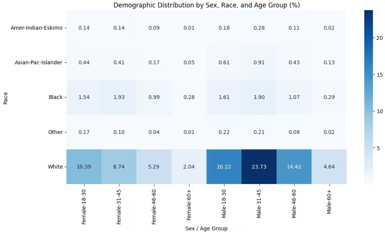
The heatmap reveals a striking imbalance, the majority of samples belong to White males aged 31–45, while groups such as Black, Islander, and Eskimo women, especially in older age brackets, are sparsely represented. A model trained on such imbalanced data tends to learn majority-group patterns more reliably, inadvertently disadvantaging underrepresented or minority group
⇒ Sampled Data Distribution Analysis Before diving into fairness metrics, it's crucial to validate whether the training and test samples represent the same population. A biased split can silently distort model behavior even before bias metrics are applied. Defined the target variable and converted it into binary
import numpy as np
from sklearn.model_selection import train_test_split
target_col = 'class'
df[target_col] = df[target_col].apply(lambda x: 1 if '>50K' in str(x) else 0)
df[target_col] = df[target_col].astype(int)
for col in df.select_dtypes(include='category').columns:
    df[col] = df[col].astype(str)
data = df.copy()
# Split features and target
X = data.drop(columns=['class'])
y = data['class']
# Identify categorical columns
cat_cols = X.select_dtypes(exclude=np.number).columns.tolist()
# Train-test split
X_train, X_test, y_train, y_test = train_test_split(
    X, y, test_size=0.2, random_state=42, stratify=y
)
for col in cat_cols:
    # Compute target mean per category on training data
    target_means = y_train.groupby(X_train[col]).mean()
    # Map to train and test
    X_train[col] = X_train[col].map(target_means)
    X_test[col] = X_test[col].map(target_means)
    # Fill unseen categories with global mean
    X_test[col].fillna(y_train.mean(), inplace=True)
python
The analysis below ensures that both data subsets are statistically consistent and free from distributional drift.
from scipy.stats import ks_2samp
num_cols = X_train.select_dtypes(include=np.number).columns.tolist()
cat_cols = X_train.select_dtypes(exclude=np.number).columns.tolist()

# Mean & Std difference check
def mean_std_diff(train, test):
    results = []
    for col in num_cols:
        t_mean, v_mean = train[col].mean(), test[col].mean()
        mean_diff = abs(t_mean - v_mean) / (abs(t_mean) + 1e-9) * 100
        results.append([col, t_mean, v_mean, mean_diff])
    return pd.DataFrame(results,
columns=['Feature','Train_Mean','Test_Mean','Mean_%Diff'])
mean_std_df = mean_std_diff(X_train, X_test)
display(mean_std_df.sort_values('Mean_%Diff', ascending=False))

# Category proportion difference
def category_proportion_diff(train, test):
    result = []
    for col in cat_cols:
        train_prop = train[col].value_counts(normalize=True)
        test_prop = test[col].value_counts(normalize=True)
        all_cats = set(train_prop.index).union(test_prop.index)
        avg_diff = np.mean([abs(train_prop.get(cat,0) -
test_prop.get(cat,0)) for cat in all_cats])*100
        result.append([col, avg_diff])
    return pd.DataFrame(result, columns=['Feature','Avg_%_Prop_Diff'])
cat_diff_df = category_proportion_diff(X_train, X_test)
display(cat_diff_df.sort_values('Avg_%_Prop_Diff', ascending=False))

# KS Test for numeric feature drift
ks_results = []
for col in num_cols:
    ks_stat, p = ks_2samp(X_train[col].dropna(), X_test[col].dropna())
    ks_results.append([col, ks_stat, p, 'Similar' if p > 0.05 else
'Different'])
ks_df = pd.DataFrame(ks_results,
columns=['Feature','KS_Stat','p_value','Interpretation'])
display(ks_df)

# PSI – Population Stability Index
def PSI(expected, actual, buckets=10):
    breakpoints = np.linspace(0, 100, buckets + 1)
    expected_perc = np.histogram(expected, bins=np.percentile(expected,
breakpoints))[0] / len(expected)
    actual_perc = np.histogram(actual, bins=np.percentile(expected,
breakpoints))[0] / len(actual)
    expected_perc = np.where(expected_perc==0, 0.0001, expected_perc)
    actual_perc = np.where(actual_perc==0, 0.0001, actual_perc)
    psi_val = np.sum((expected_perc - actual_perc) * np.log(expected_perc
/ actual_perc))
    return psi_val
psi_results = []
for col in num_cols:
    psi_val = PSI(X_train[col].dropna(), X_test[col].dropna())
    psi_results.append([col, psi_val])
psi_df = pd.DataFrame(psi_results, columns=['Feature','PSI'])
psi_df['Interpretation'] = pd.cut(
    psi_df['PSI'], bins=[-np.inf,0.1,0.25,np.inf],
    labels=['Stable','Moderate Shift','Concerning Drift']
)
display(psi_df)
python
Key Observations:
* Sample size: Train = 39,073, Test = 9,769 (80:20 split, stratified by class).
* Numerical stability: All six numeric features show consistent distributions with < 15% mean difference. Slight variations in capital-loss (13.6%) and capital-gain (10.2%) are acceptable, indicating stable central tendency and spread.
* Category proportion difference: All categorical variables show <1% average difference, with small shifts in age_group (0.61%) and relationship (0.30%), well within acceptable limits.
* KS Test & PSI: All numerical features passed KS (p > 0.05) and PSI < 0.1, confirming no statistically significant drift or population shift.
* Correlation consistency: Average difference in inter-feature correlations <0.01, suggesting relationships among features remain steady across splits.
text⇒ Model Fairness Auditing We have used LightGBM to train out model and obtained following results:
# LightGBM model with strong baseline hyperparameters

params = {
    'objective': 'multiclass' if len(np.unique(y)) > 2 else 'binary',
    'num_class': len(np.unique(y)) if len(np.unique(y)) > 2 else 1,
    'boosting_type': 'gbdt',
    'learning_rate': 0.05,
    'n_estimators': 500,
    'max_depth': -1,
    'num_leaves': 31,
    'subsample': 0.8,
    'colsample_bytree': 0.8,
    'reg_alpha': 0.1,
    'reg_lambda': 0.1,
    'random_state': 42
}


# Train model
model = lgb.LGBMClassifier(**params)
model.fit(X_train, y_train)


# Predictions
y_pred = model.predict(X_test)


# Evaluation
print("Accuracy:", accuracy_score(y_test, y_pred))
print("Precision:", precision_score(y_test, y_pred, average='weighted'))
print("Recall:", recall_score(y_test, y_pred, average='weighted'))
print("F1 Score:", f1_score(y_test, y_pred, average='weighted'))
print("\nConfusion Matrix:\n", confusion_matrix(y_test, y_pred))

python
Accuracy: 0.8777766403930801
Precision: 0.8735920264166155
Recall: 0.8777766403930801
F1 Score: 0.8738250433951856
Confusion Matrix:
[[7027 404]
[ 790 1548]]
textEven though our LightGBM model achieves ~87.7% accuracy and balanced precision/recall, performance alone doesn't guarantee fairness.
An AI model can perform well overall yet systematically disfavor certain subgroups, a phenomenon often hidden behind aggregate scores.
To uncover this, we audit fairness of gender and race, two sensitive attributes in the Adult Income dataset using group-level metrics and the Disparate Impact (DI) measure.
The Disparate Impact (DI) quantifies whether different demographic groups receive favorable outcomes (positive predictions) at comparable rates. A DI value below 0.8 typically indicates potential bias or unfair treatment in model predictions.
Results Overview Fairness by Sex
| sex | Selection Rate | TPR | FPR | Count |
|---|---|---|---|---|
| Female | 0.083 | 0.598 | 0.019 | 3259 |
| Male | 0.258 | 0.674 | 0.077 | 6510 |
Fairness by Race
| race | Selection Rate | TPR | FPR | Count |
|---|---|---|---|---|
| Amer-Indian-Eskimo | 0.062 | 0.462 | 0.000 | 96 |
| Asian-Pac-Islander | 0.248 | 0.671 | 0.096 | 311 |
| Black | 0.084 | 0.535 | 0.014 | 968 |
| Other | 0.073 | 0.600 | 0.000 | 82 |
| White | 0.214 | 0.671 | 0.060 | 8312 |
Disparate Impact (DI)
| Protected Attribute | Disparate Impact (DI) |
|---|---|
| sex | 0.322 |
| race | 0.250 |
The audit reveals substantial fairness concerns in the model, particularly with respect to sex and race. Both attributes exhibit Disparate Impact values far below the 0.8 threshold, indicating unequal treatment.
Let's undergo bias mitigation using reweighing to ensure more equitable and trustworthy decision-making.
# Identify Sensitive Attribute and Define Groups
sensitive_attr = 'sex'
privileged = 'Male'
unprivileged = 'Female'


train_df = X_train.copy()
train_df[target_col] = y_train


# Count Observed Frequencies for Each Group–Label Pair
# Eg: (Male, >50K), (Male, <=50K), (Female, >50K), (Female, <=50K)
# This gives us the REAL (observed) distribution in the data.
group_counts = train_df.groupby([sensitive_attr, target_col]).size().reset_index(name='count')


# Compute overall percentages:
#    - What % of people are Male vs Female?
#    - What % of people earn >50K vs <=50K?
P_y = train_df[target_col].value_counts(normalize=True)
P_a = train_df[sensitive_attr].value_counts(normalize=True)


# Compute REAL probability of each (group, label) pair.
# Eg: P(Male, >50K)and so on..
P_a_y = (group_counts.set_index([sensitive_attr, target_col])['count'] / len(train_df))


#Compute what the probabilities should be if gender and income were totally independent.
# This represents an "unbiased world" expectation.
expected_P_a_y = {
    (a, y): P_a[a] * P_y[y] for a in P_a.index for y in P_y.index
}


# Compute reweighing factor: w = expected / observed
# If a group appears TOO MUCH → weight < 1 (down-weight), if a group appears TOO LITTLE → weight > 1 (boost)
weights = {}
for a in P_a.index:
    for yval in P_y.index:
        obs = P_a_y.get((a, yval), 1e-6)
        exp = expected_P_a_y[(a, yval)]
        weights[(a, yval)] = exp / obs


# Assign each row its calculated weight based on its group
train_df['weight'] = [
    weights.get((a, y), 1.0)
    for a, y in zip(train_df[sensitive_attr], train_df[target_col])
]


sample_weights = train_df['weight'].values


# Target encoding (same as before)
for col in cat_cols:
    target_means = y_train.groupby(X_train[col]).mean()
    X_train[col] = X_train[col].map(target_means)
    X_test[col] = X_test[col].map(target_means)
    X_test[col].fillna(y_train.mean(), inplace=True)


# Train LightGBM using weights
params = {
    'objective': 'binary',
    'boosting_type': 'gbdt',
    'learning_rate': 0.05,
    'n_estimators': 500,
    'num_leaves': 31,
    'subsample': 0.8,
    'colsample_bytree': 0.8,
    'reg_alpha': 0.1,
    'reg_lambda': 0.1,
    'random_state': 42,
}


model = lgb.LGBMClassifier(**params)
model.fit(X_train, y_train, sample_weight=sample_weights)


y_pred = model.predict(X_test)


# Evaluation
print(" Model Evaluation with Reweighing:")
print("Accuracy :", accuracy_score(y_test, y_pred))
print("Precision:", precision_score(y_test, y_pred))
print("Recall   :", recall_score(y_test, y_pred))
print("F1 Score :", f1_score(y_test, y_pred))

python
Accuracy : 0.8706111167980346
Precision: 0.7973421926910299
Recall : 0.6159110350727117
F1 Score : 0.6949806949806949
Fairness by Sex
| sex | Selection Rate | TPR | FPR | Count |
|---|---|---|---|---|
| Female | 0.122 | 0.717 | 0.048 | 3259 |
| Male | 0.215 | 0.593 | 0.050 | 6510 |
Disparate Impact (DI)
| Protected Attribute | Disparate Impact (DI) |
|---|---|
| sex | 0.567 |
| race | 0.364 |
We can see that female selection rate increased, male selection rate balanced downward, error rates (TPR/FPR) became more symmetric.
The model is now meaningfully less discriminatory, though DI is still not perfect, showing that fairness mitigation is an iterative process.
Closing Thoughts
AI is no longer a distant innovation, it's the invisible engine shaping decisions that touch every aspect of our lives.
As we've seen, bias in AI isn't always born of bad intent; it often stems from blind spots in data, in design or in governance but acknowledging those blind spots is the first step toward progress.
Responsible AI isn't about perfection, it's about transparency, accountability and continuous improvement. Building ethical AI requires more than good algorithms; it demands good judgment. It means embedding fairness checks into every stage, from data collection to deployment and fostering collaboration between technologists, domain experts and ethicists. Because in the end, the real measure of AI's success isn't how intelligent it becomes but how wisely and fairly we choose to use it.
The future of AI will not be defined by its capability, but by its conscience.


